Lesson 4 - Your First R Code
• How to work with RStudio.
• How to write and run R code.
• How to create simple plots.
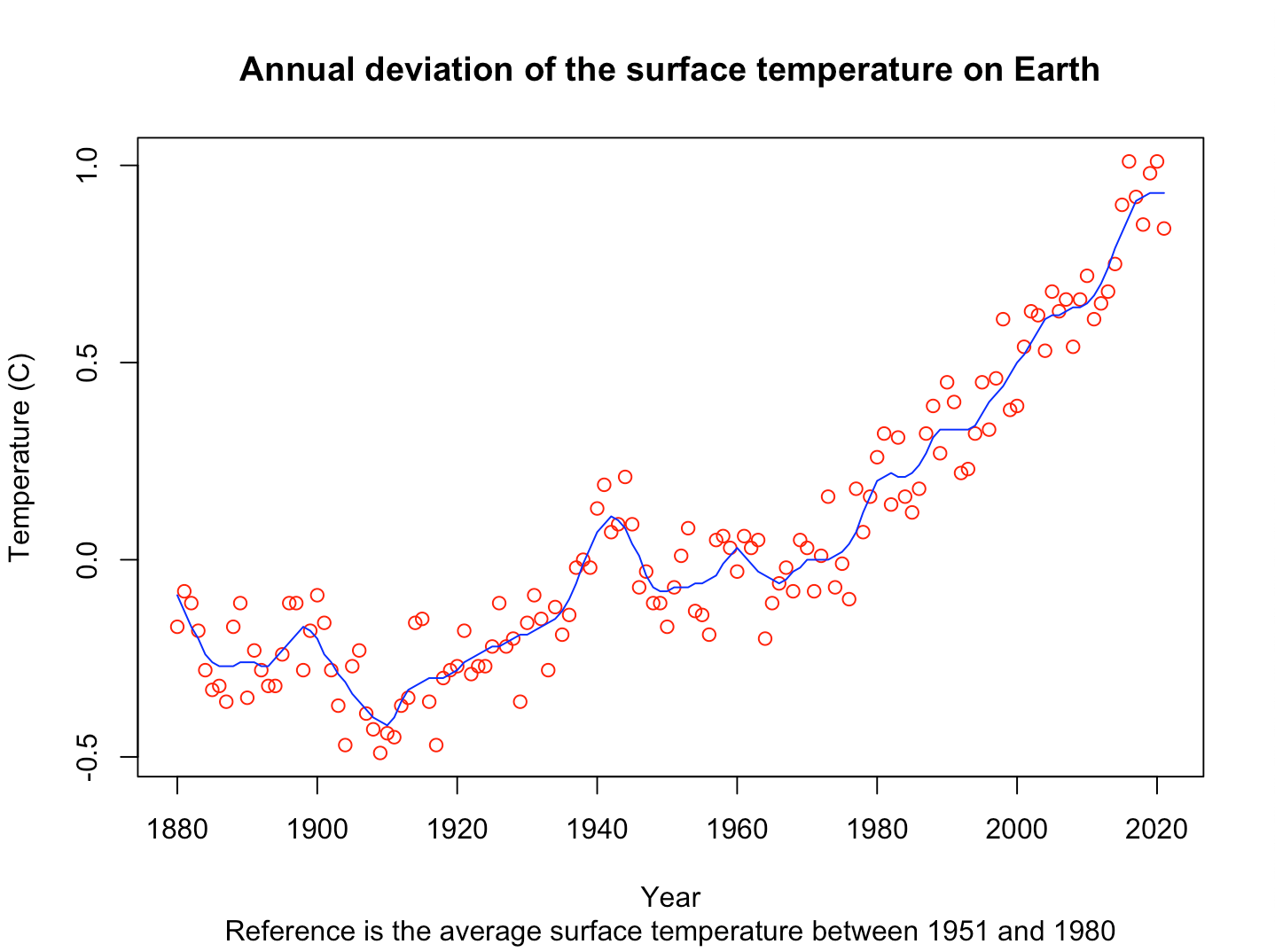
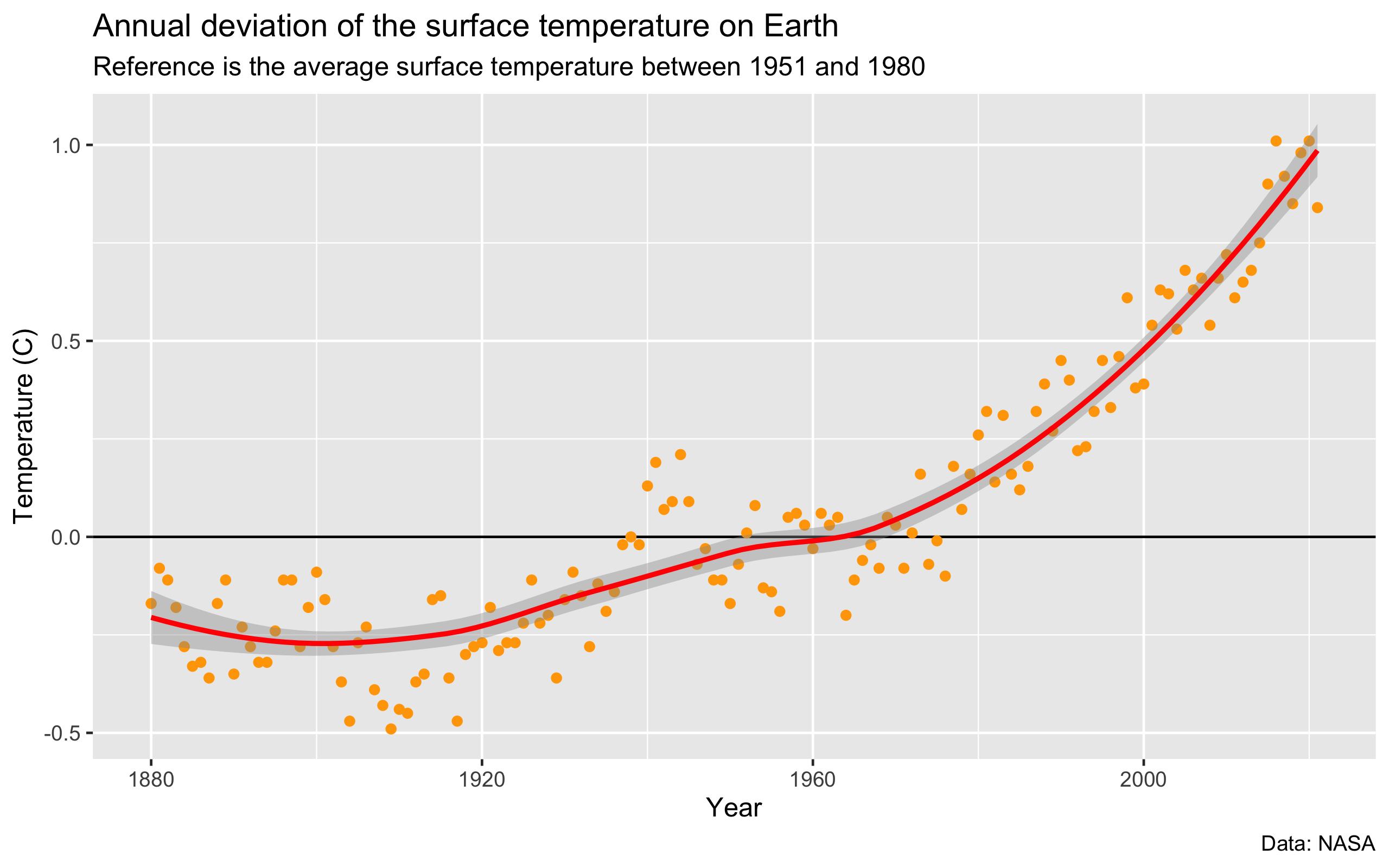
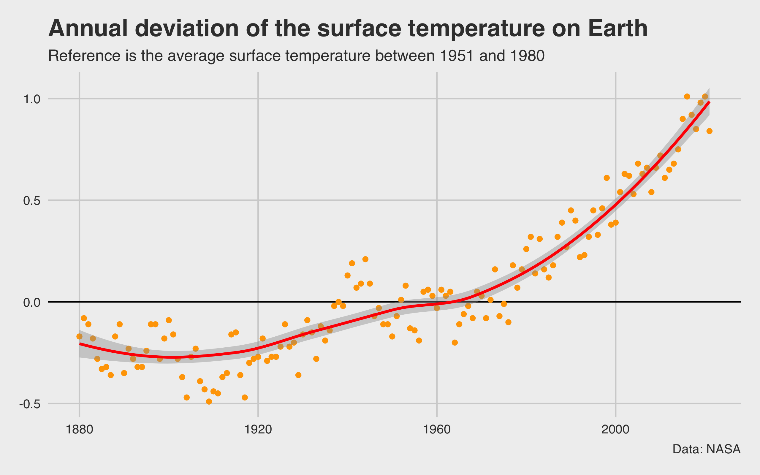
It is now time to meet R and RStudio. This is where the fun really begins! With a few lines of code, at the end of the lesson you will have created this plot.
4.1 Let’s get started
Open RStudio. A window appears.
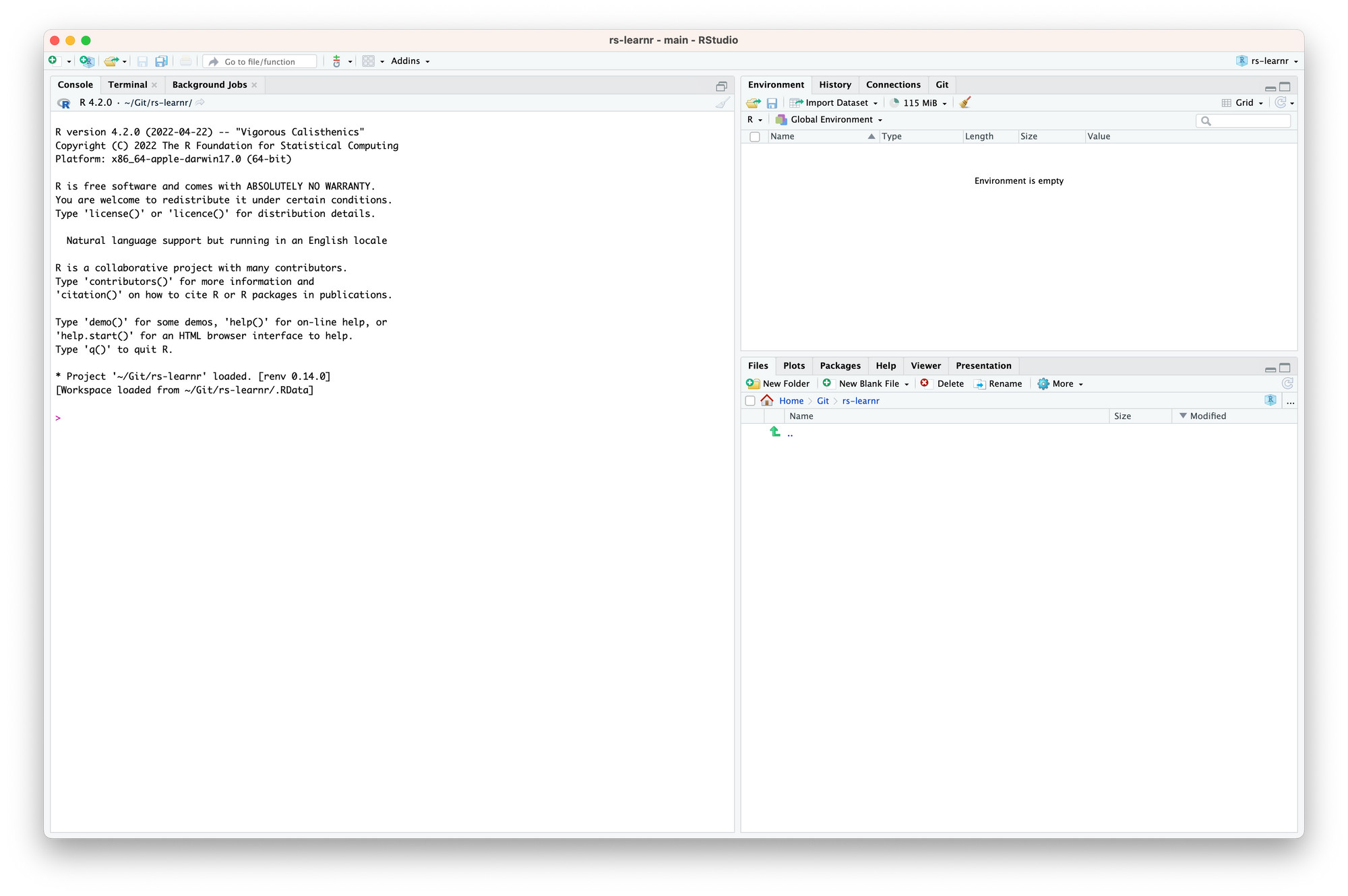
RStudio can feel intimidating — but is really not. In a latter lesson, you will learn in more detail about how it works. For the time being, we will use a small subset of its features.
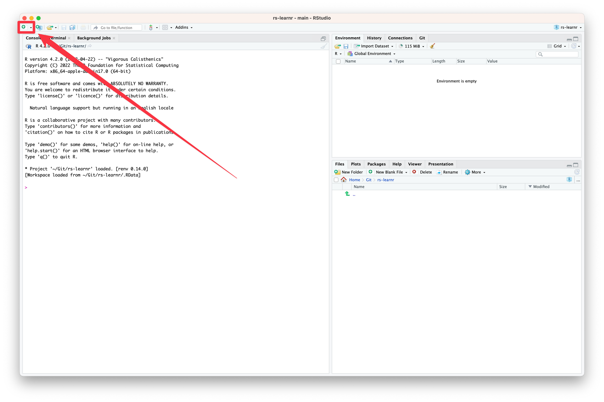
We need to create a file to write and run our code.
Click on the + icon to create a new file.
In the menu, choose R Script.
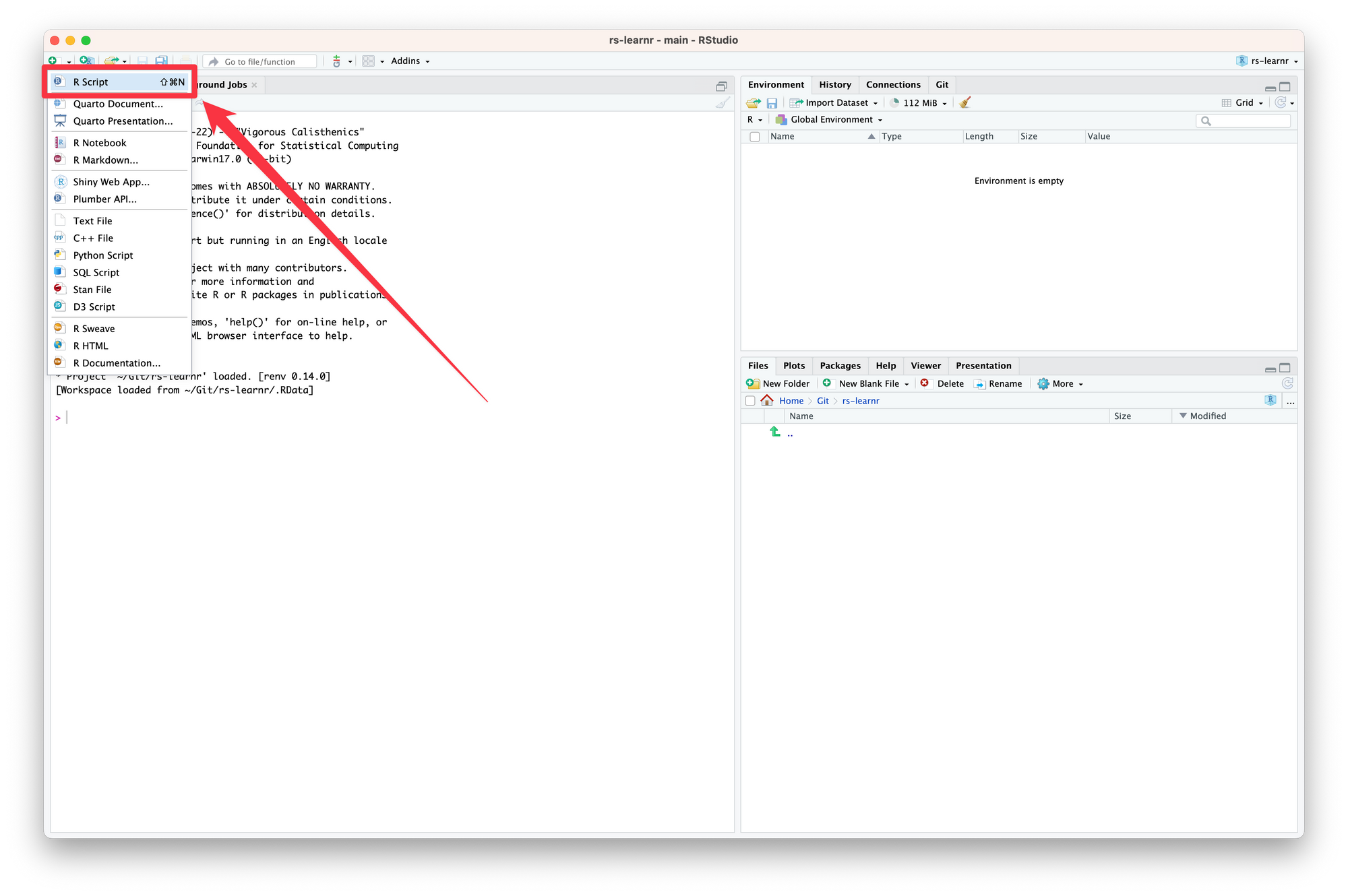
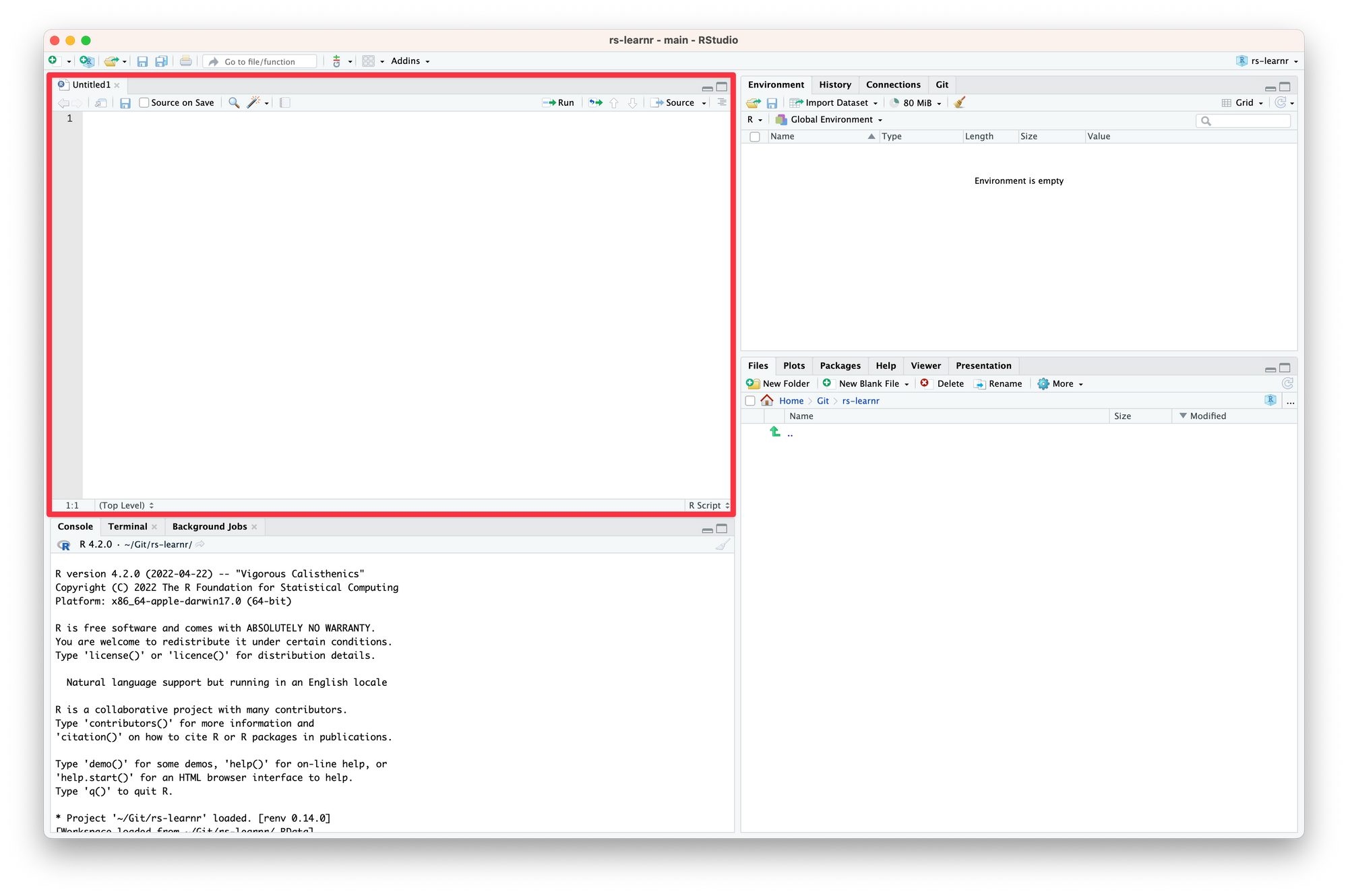
A new pane has appeared. This is where we will write our code.
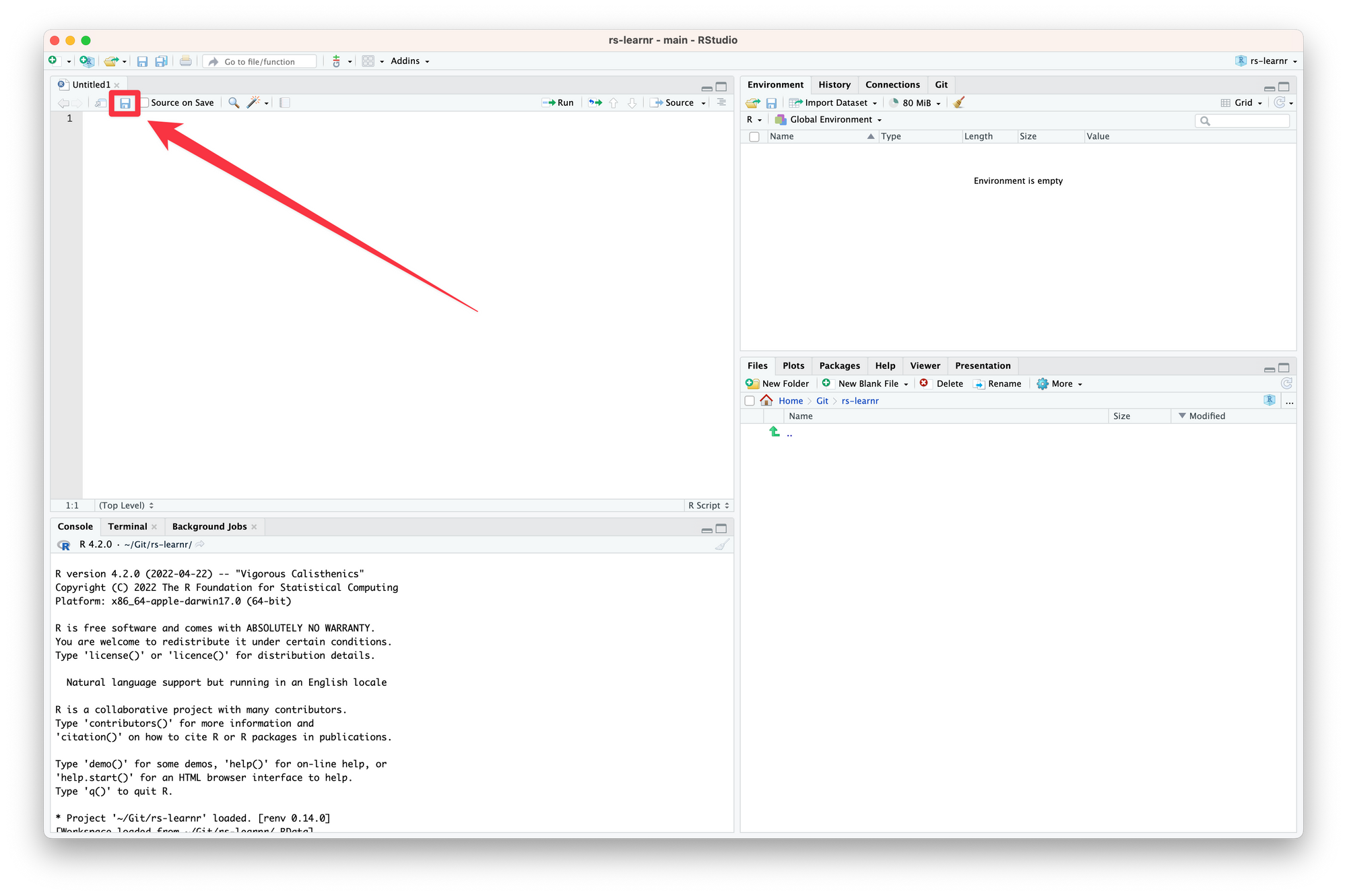
Save the file by clicking on the floppy disk icon. Name it anything you want, and make sure it ends with .R. You can save it anywhere you like on your computer.
We can now write our first line of R code!
4.2 Your first code
For this lesson, I created a small dataset for you. It is based on a simple climate change dataset from NASA.
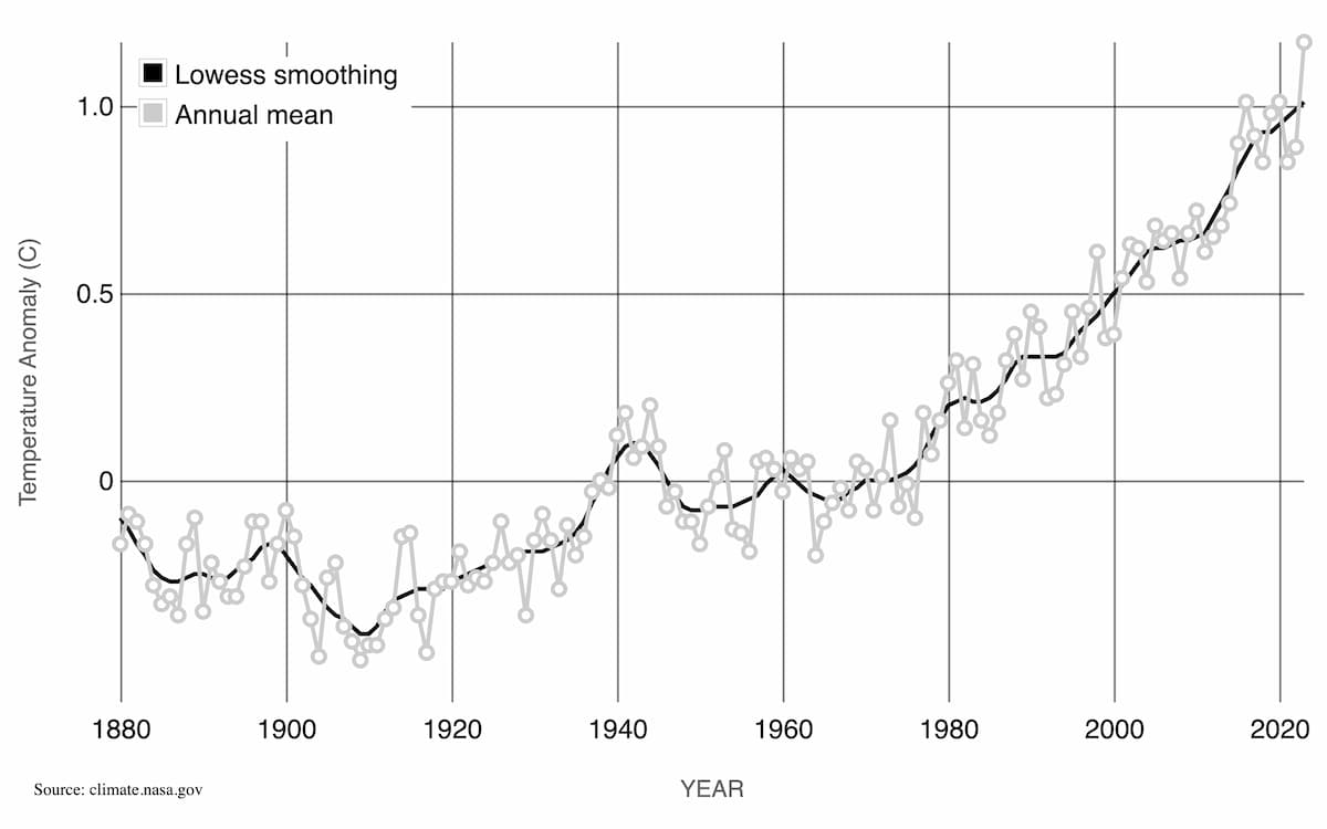
The data are annual deviations of the average Earth surface temperature from 1880 to 2021 compared to the Earth surface temperature averaged between 1951 and 1980. A negative value, for instance -0.6, means that the average surface temperature was 0.6 °C lower for that year compared to the 1951-1980 average. A positive value, for instance 0.8, means that the average surface temperature was 0.8 °C higher for that year compared to the 1951-1980 average.
To work with the dataset, we need to import it. The dataset is a CSV file. I uploaded it on a GitHub repository.
We could download the CSV file manually, and then write code to import its content. But we can streamline the process by writing code that imports the file directly.
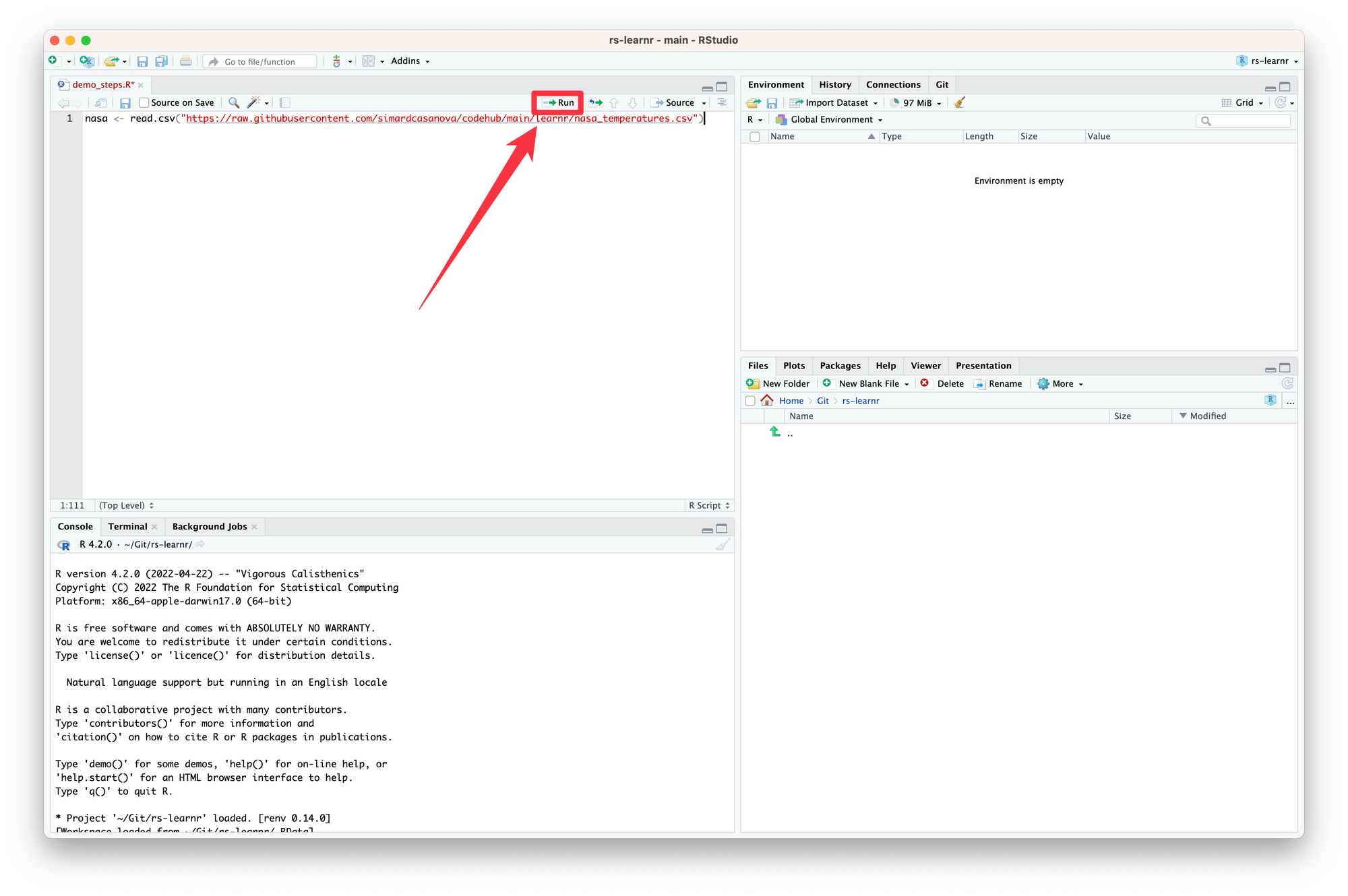
nasa <- read.csv("https://course-r-getting-started.simardcasanova.net/content/files/2024/03/nasa_temperatures.csv")Let’s break down the code we just wrote.
read.csv() is a base R function that imports CSV files. The function can import CSV files that are stored locally or online. In our case, the file is stored online.
The URL in quote marks "https://course-r-getting-started.simardcasanova.net/content/files/2024/03/nasa_temperatures.csv" is where the CSV file is located.
nasa is a variable that stores the dataset we will import from the CSV file into R. In R, datasets usually take the form of what R calls data frames. Data frames are a special type of variable designed to store data structured in rows and columns.
Last but not least, <-. You will use this symbol a lot. It’s a pivotal piece of R. This symbol is the assignment operator. Its role is to tell R that the variable nasa stores whatever is on the right side of it. In our case, we tell R to assign to nasa the result of read.csv() — i.e. the content of the CSV file.
4.3 Run your first code
You have your first code! Now we need to run it so that R executes the code we just wrote.
In RStudio, you can run your code in different ways.
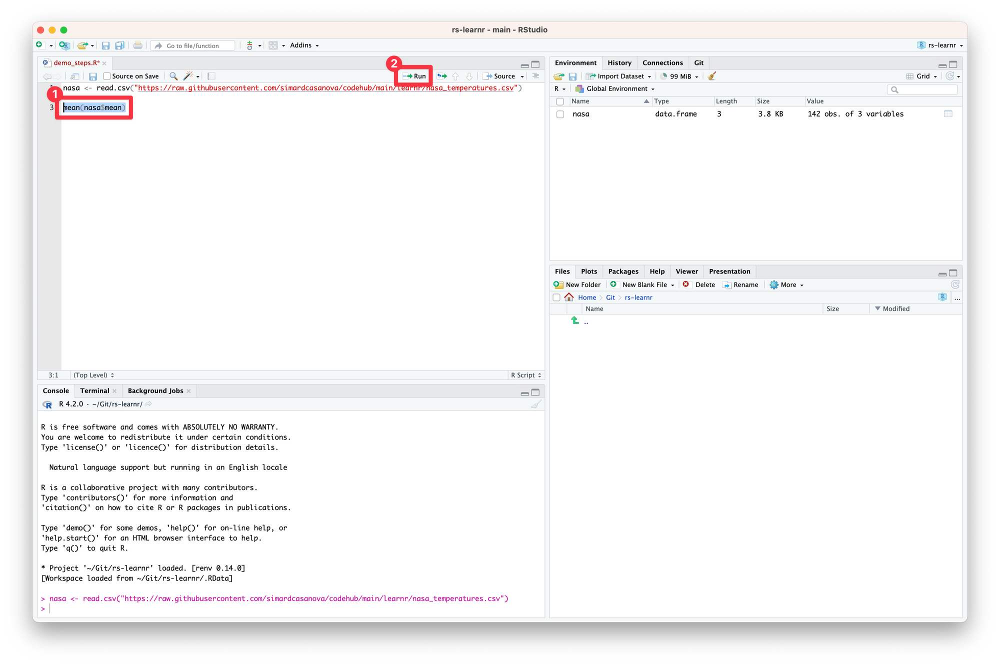
The simplest way is to click on the Run button. Put the cursor on the line we just wrote and click Run.
Congratulations! You just ran your first R code.
By default, clicking on Run runs the line your cursor is on. If you click the small arrow at the right of the Run button, you can find the keyboard shortcut to run the current line. This keyboard shortcut is a great time saver.
To run the whole file, select all its lines and click Run (or use the keyboard shortcut).
You may have noticed that a few things have changed in RStudio. For now, let’s focus on the console (1) and on the environment tab (2).
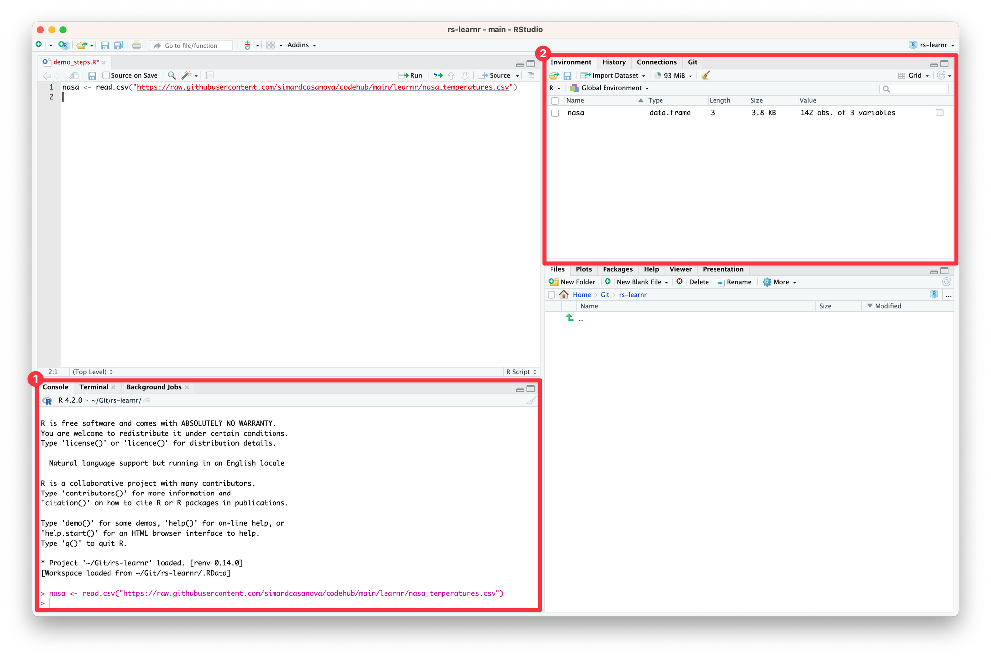
The console (1) shows which code ran and provides useful output — in particular, errors. Luckily for us, the console shows no error. It means the code ran successfully.
In the Environment tab (2), a line named nasa appeared. The line means that R successfully imported the CSV file into the nasa variable—exactly as we instructed. We can see that nasa is a variable of type data.frame. The data frame nasa contains 142 observations (= rows) of 3 variables (= columns).
4.4 Meet the power of RStudio
We have imported our dataset. Now, we can work on it. RStudio offers a lot of features that make working with R a breeze. Let’s look at the data we just imported.
Click the View button in the Environment tab.
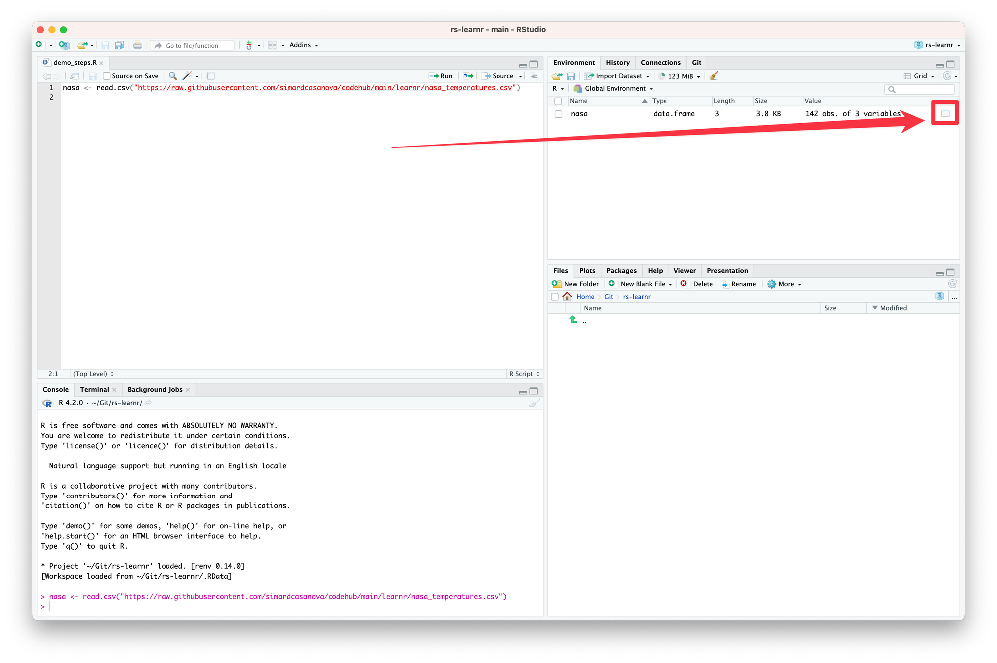
RStudio opens a tab that displays the data frame.
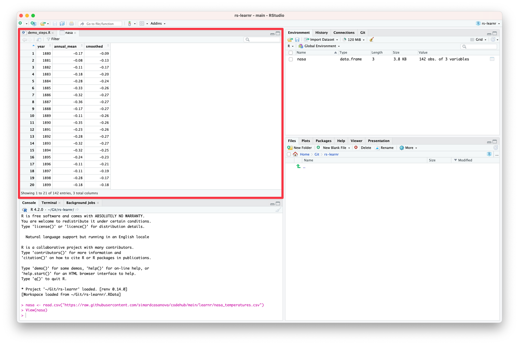
Thanks to the View tab, we can take a quick look at nasa to make sure that everything has been imported correctly. View tabs are read only: you cannot edit the data they display. To edit the data, you need to write R code to edit the underlying data frames—something you will learn in a later lesson.
Let’s compute the mean of the Earth average annual surface temperature. Write the following code in the R file. Do not copy and paste it, type it. Do not run it yet.
mean(nasa$annual_mean)Right after you wrote $, something like this appeared.
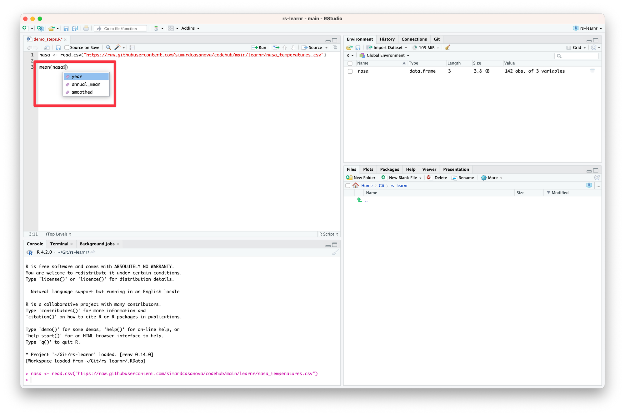
This feature is called autocompletion. RStudio lists all the columns it has detected automatically inside nasa for us to pick one. Autocompletion is another massive time saver. It makes writing code easier and faster. It reduces the likelihood of introducing errors. And it gives useful information on the data we are working with.
RStudio tells us that nasa is made of three variables: year, annual_mean and smoothed.
Now, let’s run the code we just wrote—but don’t use the Run button yet. First, select the code we added. Only then, click Run—or, even better, use the keyboard shortcut associated with Run Selected Line(s).
Something new appeared in the console.
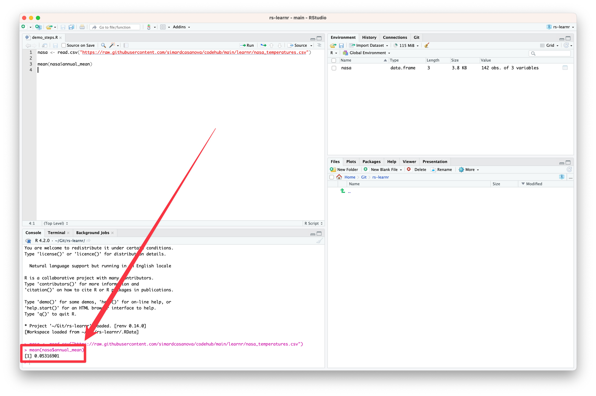
The console outputs the results of the code we just ran—the mean of annual_mean computed over all the years in the data frame. In my computer, the value is 0.05316901. It means that on average, between 1880 and 2021 the surface temperature is 0.05 °C over the surface temperature averaged between 1951 and 1980.
4.5 Plotting
We have computed a mean. But averaging deviations on such a large period (1880-2021) is not that informative. We know that surface temperature only started to rise recently. Could we see this recent rise on a plot?
R has built-in plotting capabilities. They are not great, but they will be enough for now. You will learn in a later lesson more powerful plotting tools.
Let’s add this code to the file.
plot(
  nasa$year,
  nasa$annual_mean
)
This code creates a plot with nasa$year as the \( x \) axis and nasa$annual_mean as the \( y \) axis.
Run the code. Congratulations! You created your first plot with R.
RStudio refocused on the Plots tab. This tab conveniently shows the plots we create.
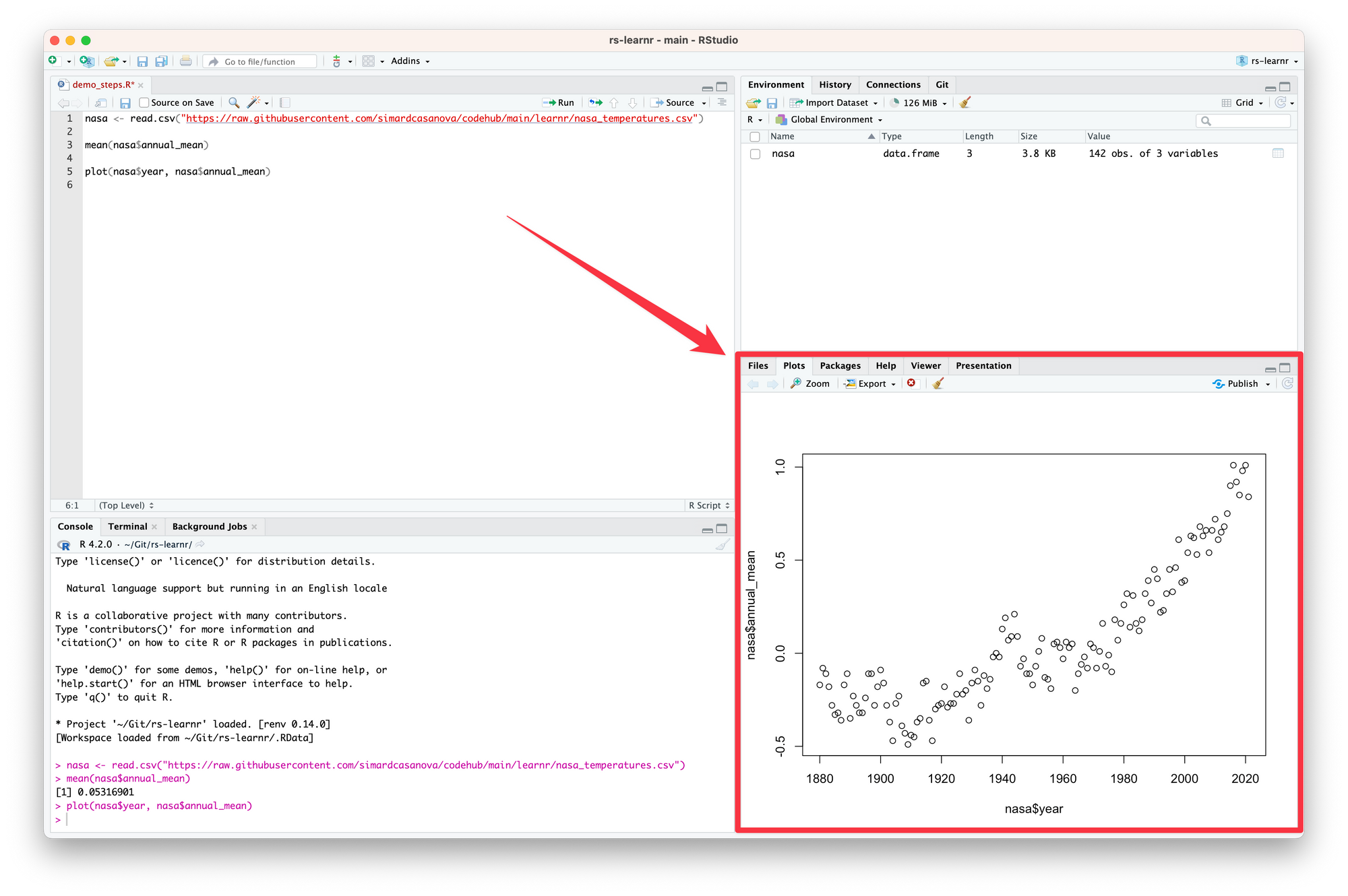
The plot shows that the surface temperature started to rise around the 1970s.
Let’s recompute the average deviation, but this time only for the 1980-2021 period. To compute a mean on a subset of the data frame, we need to tell R to restrict the data frame to the years that comes after 1980 (1980 excluded).
mean(nasa[nasa$year > 1980, ]$annual_mean)The part between brackets tells R to take the data frame nasa, and to only keep the rows where year is strictly larger than 1980. mean() will be computed on the values of annual_mean stored in this smaller data frame.
At this point, you may think that the last code we wrote is kind of ugly. Or at the very least, hard to read. Personally, I think it’s both. In a latter lesson, we will introduce the Tidyverse. Thanks to it, we will be able to write clearer, prettier, and more readable code.
For the time being, let’s keep working with what we have. The console tells us that the average yearly deviation after 1980 is around 0.5 °C.
4.6 A prettier—ish plot
Looking at the plot, aren’t you tempted to draw a smoothed curve between the dots? Because I definitely am. Luckily for us, NASA provided a variable smoothed we can use to draw this curve.
Let’s use smoothed to add a curve that smooths the points. We can also add colors to distinguish the dots and the curve. Run both lines.
plot(
  nasa$year,
  nasa$annual_mean,
  col = "red"
)
lines(
  nasa$year,
  nasa$smoothed,
  col = "blue"
)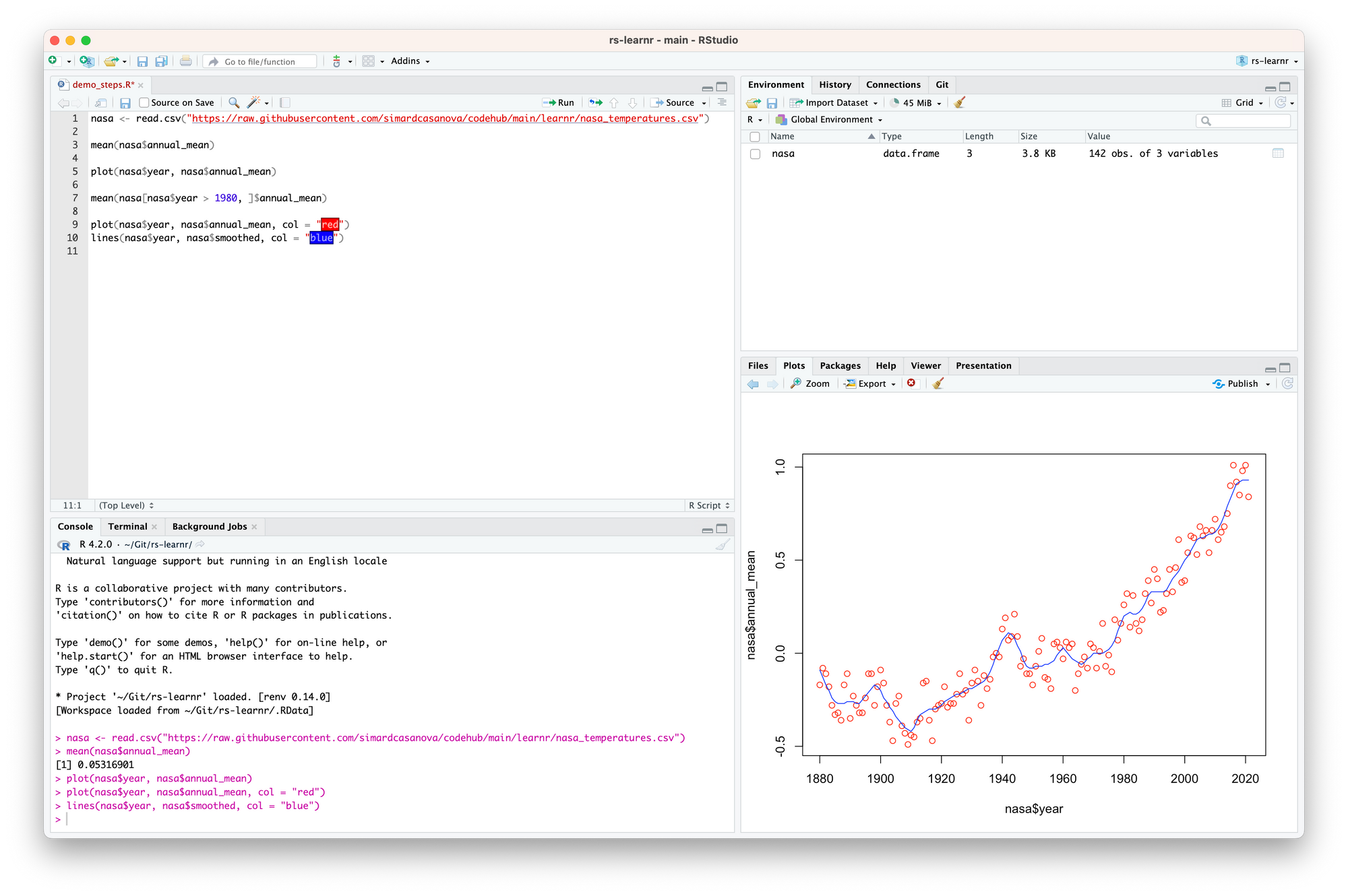
col tells R to color the dots in red and the curve in blue.
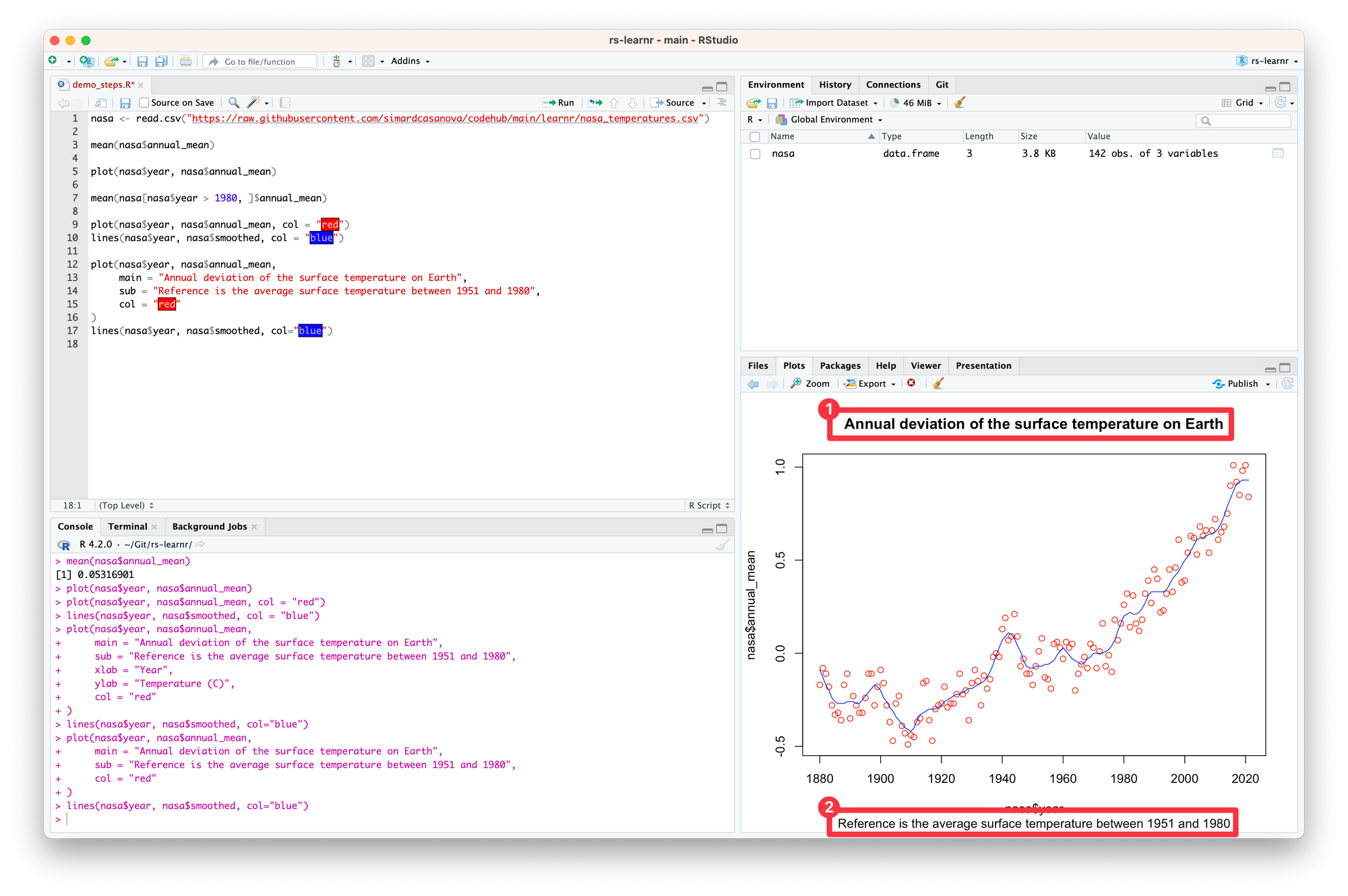
Another thing I am tempted to do is to make the plot more informative. In my opinion, it needs a title (1) and a subtitle (2).
plot(
  nasa$year,
  nasa$annual_mean,
  main = "Annual deviation of the surface temperature on Earth",
  sub = "Reference is the average surface temperature between 1951 and 1980",
  col = "red"
)
lines(
  nasa$year,
  nasa$smoothed,
  col="blue"
)
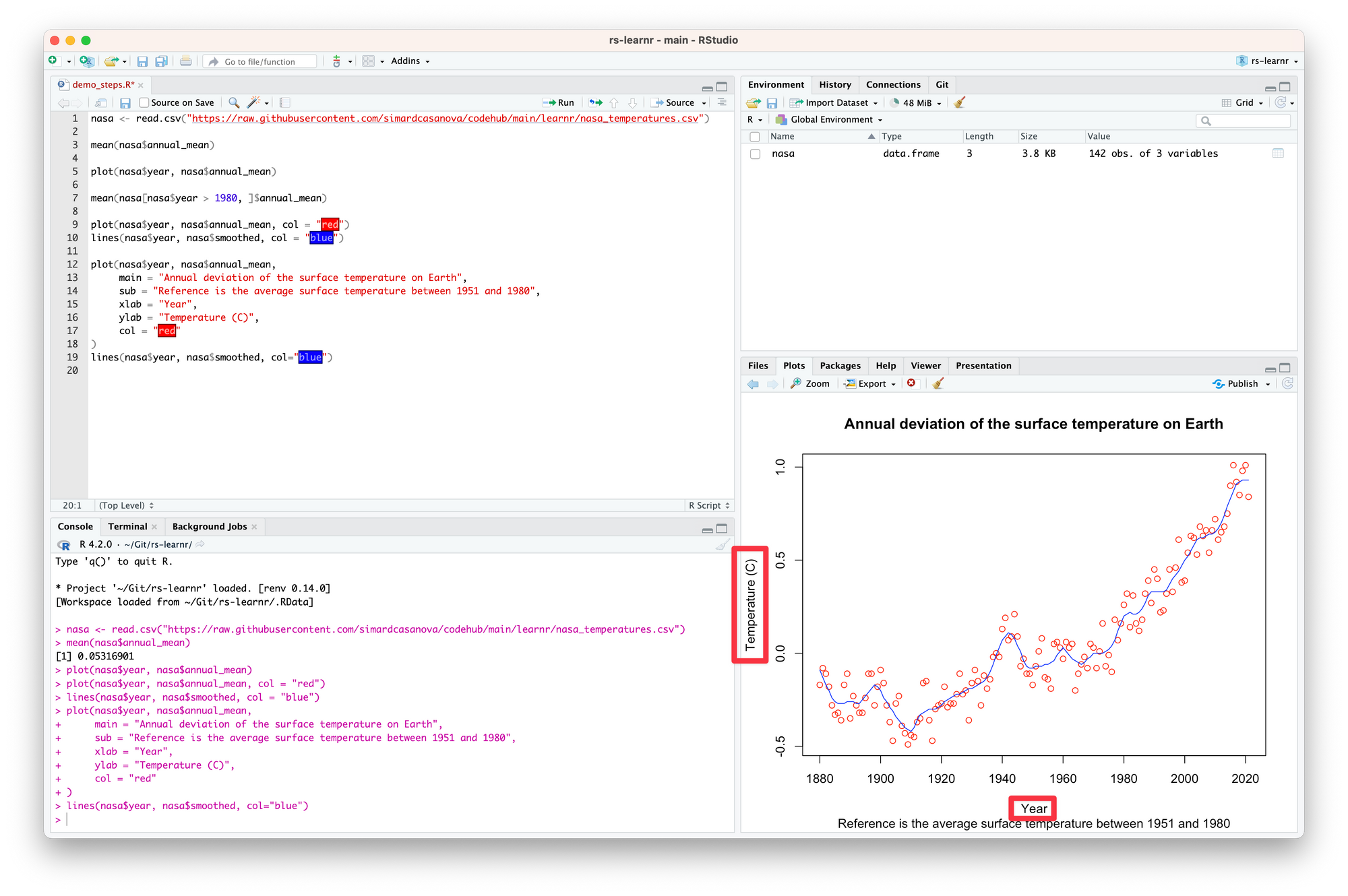
I am also tempted to change the labels on the axes. Currently, they are not informative enough.
plot(
  nasa$year,
  nasa$annual_mean,
  main = "Annual deviation of the surface temperature on Earth",
  sub = "Reference is the average surface temperature between 1951 and 1980",
  xlab = "Year",
  ylab = "Temperature (C)",
  col = "red"
)
lines(
  nasa$year,
  nasa$smoothed,
  col="blue"
)
We now have a marginally less ugly plot. That being said, we will probably agree that the plot is still not that good-looking. Thanks to the more advanced plotting capabilities we will see in a latter lesson, you will be able to produce much fancier plots.
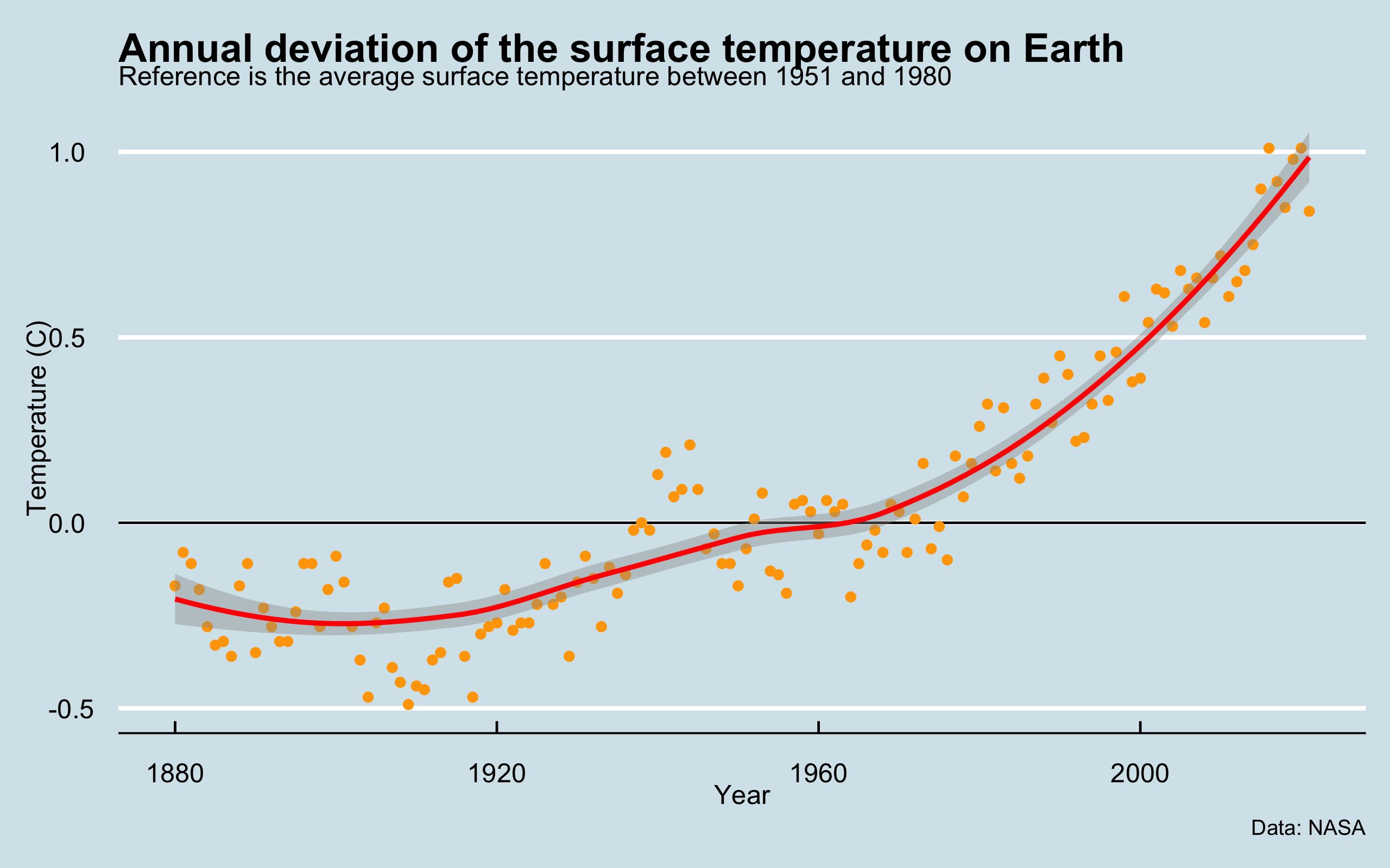
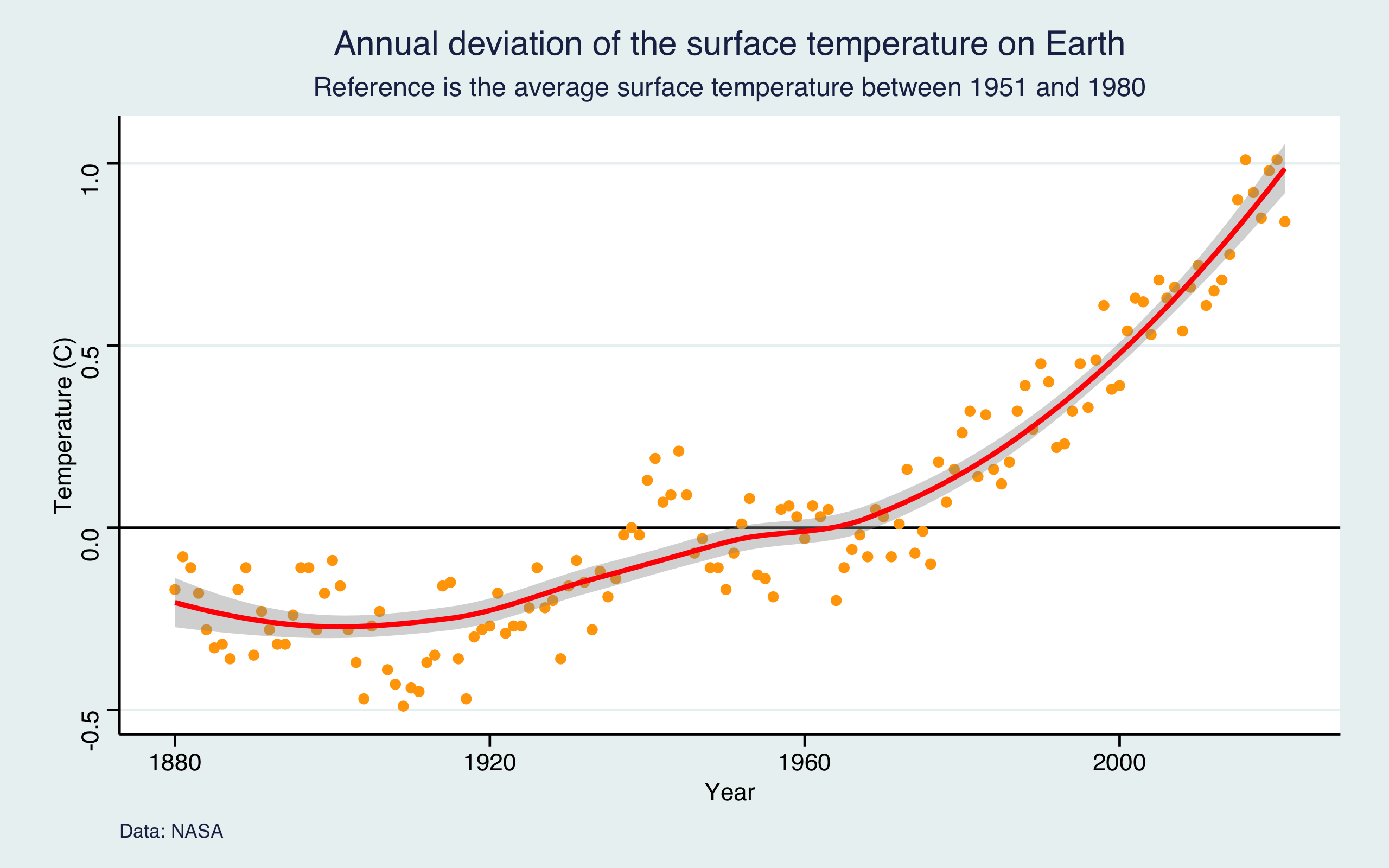
We even have the Stata fans covered.
That’s it for this lesson!
You have met R and RStudio. In theory, you could start to work on your data right away. But what about these fancy plots? What about the Tidyverse? What about this more readable code? What about importing Excel files? What about linear regressions? You will learn these things, and so much more, in the remaining lessons of the course.
If you have already purchased the online course, you can go to the next lesson.